Benchmarking large-scale integration#
Here we walkthrough applying the integration benchmarking metrics on a dataset of non-small cell lung cancer from the following paper:
Salcher, S., Sturm, G., Horvath, L., Untergasser, G., Kuempers, C., Fotakis, G., … & Trajanoski, Z. (2022). High-resolution single-cell atlas reveals diversity and plasticity of tissue-resident neutrophils in non-small cell lung cancer. Cancer Cell.
This dataset contains ~900,000 cells, so here we demonstrate the scalbility of the metrics here on large data.
import numpy as np
import scanpy as sc
from scvi.data import cellxgene

from scib_metrics.benchmark import Benchmarker, BioConservation, BatchCorrection

%matplotlib inline
Load and preprocess data#
url = "https://cellxgene.cziscience.com/e/232f6a5a-a04c-4758-a6e8-88ab2e3a6e69.cxg/"
adata = cellxgene(url, filename="luca.h5ad", save_path="data/")
adata
AnnData object with n_obs × n_vars = 892296 × 17811
    obs: 'sample', 'uicc_stage', 'ever_smoker', 'age', 'donor_id', 'origin', 'dataset', 'ann_fine', 'cell_type_predicted', 'doublet_status', 'leiden', 'n_genes_by_counts', 'total_counts', 'total_counts_mito', 'pct_counts_mito', 'ann_coarse', 'cell_type_tumor', 'tumor_stage', 'EGFR_mutation', 'TP53_mutation', 'ALK_mutation', 'BRAF_mutation', 'ERBB2_mutation', 'KRAS_mutation', 'ROS_mutation', 'origin_fine', 'study', 'platform', 'cell_type_major', 'suspension_type', 'assay_ontology_term_id', 'cell_type_ontology_term_id', 'development_stage_ontology_term_id', 'disease_ontology_term_id', 'self_reported_ethnicity_ontology_term_id', 'is_primary_data', 'organism_ontology_term_id', 'sex_ontology_term_id', 'tissue_ontology_term_id', 'cell_type', 'assay', 'disease', 'organism', 'sex', 'tissue', 'self_reported_ethnicity', 'development_stage'
    var: 'is_highly_variable', 'mito', 'n_cells_by_counts', 'mean_counts', 'pct_dropout_by_counts', 'total_counts', 'feature_is_filtered', 'feature_name', 'feature_reference', 'feature_biotype'
    uns: '_scvi', 'ann_fine_colors', 'batch_condition', 'cell_type_major_colors', 'cell_type_ontology_term_id_colors', 'cell_type_predicted_colors', 'dataset_colors', 'default_embedding', 'hvg', 'leiden_colors', 'neighbors', 'origin_colors', 'platform_colors', 'schema_version', 'title', 'umap'
    obsm: 'X_scANVI', 'X_scVI', 'X_umap'
    layers: 'count', 'counts_length_scaled'
    obsp: 'connectivities', 'distances'
sc.pp.subsample(adata, n_obs=500_000)
# Number of unique cell types
adata.obs["cell_type"].nunique()
33
adata.var["highly_variable"] = np.asarray(adata.var["is_highly_variable"].astype(bool))
sc.tl.pca(adata)
“Run” methods#
The authors used scVI and scANVI in their manuscript, and these embeddings are already stored in the AnnData object. We can use these to run the metrics.
scVI#
adata.obsm["scVI"] = adata.obsm["X_scVI"]
scANVI#
adata.obsm["scANVI"] = adata.obsm["X_scANVI"]
Perform the benchmark#
Here we use a custom nearest neighbor function to speed up the computation of the metrics. This is not necessary, but can be useful for large datasets.
In particular we use faiss, which can be accelerated with a GPU.
This can be installed as
conda install -c conda-forge faiss-gpu
When using approximate nearest neighbors, an issue can arise where each cell does not get a unique set of K neighbors. This issue happens with faiss hnsw below, so we use the brute force method instead, which is still faster than pynndescent approximate nearest neighbors on CPU.
import faiss

from scib_metrics.nearest_neighbors import NeighborsResults


def faiss_hnsw_nn(X: np.ndarray, k: int):
    """Gpu HNSW nearest neighbor search using faiss.

    See https://github.com/nmslib/hnswlib/blob/master/ALGO_PARAMS.md
    for index param details.
    """
    X = np.ascontiguousarray(X, dtype=np.float32)
    res = faiss.StandardGpuResources()
    M = 32
    index = faiss.IndexHNSWFlat(X.shape[1], M, faiss.METRIC_L2)
    gpu_index = faiss.index_cpu_to_gpu(res, 0, index)
    gpu_index.add(X)
    distances, indices = gpu_index.search(X, k)
    del index
    del gpu_index
    # distances are squared
    return NeighborsResults(indices=indices, distances=np.sqrt(distances))


def faiss_brute_force_nn(X: np.ndarray, k: int):
    """Gpu brute force nearest neighbor search using faiss."""
    X = np.ascontiguousarray(X, dtype=np.float32)
    res = faiss.StandardGpuResources()
    index = faiss.IndexFlatL2(X.shape[1])
    gpu_index = faiss.index_cpu_to_gpu(res, 0, index)
    gpu_index.add(X)
    distances, indices = gpu_index.search(X, k)
    del index
    del gpu_index
    # distances are squared
    return NeighborsResults(indices=indices, distances=np.sqrt(distances))
import time

adata.obsm["Unintegrated"] = adata.obsm["X_pca"]

biocons = BioConservation(isolated_labels=False)

start = time.time()
bm = Benchmarker(
    adata,
    batch_key="sample",
    label_key="cell_type",
    embedding_obsm_keys=["Unintegrated", "scANVI", "scVI"],
    pre_integrated_embedding_obsm_key="X_pca",
    bio_conservation_metrics=biocons,
    batch_correction_metrics=BatchCorrection(),
    n_jobs=-1,
)
bm.prepare(neighbor_computer=faiss_brute_force_nn)
bm.benchmark()
end = time.time()
print(f"Time: {int((end - start) / 60)} min {int((end - start) % 60)} sec")
Time: 20 min 45 sec
Visualize the results#
bm.plot_results_table()
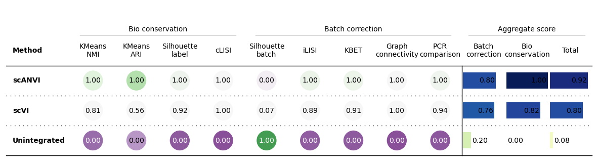
<plottable.table.Table at 0x7f2642db39a0>
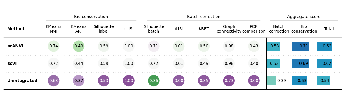
bm.plot_results_table(min_max_scale=False)
<plottable.table.Table at 0x7f2714881870>
We can also access the underlying dataframes to print the results ourselves.
from rich import print

df = bm.get_results(min_max_scale=False)
print(df)
                    KMeans NMI        KMeans ARI  Silhouette label  \
Embedding
Unintegrated          0.630967          0.372678          0.531423
scANVI                0.744273          0.485717          0.594908
scVI                  0.722253          0.435955          0.590104
Metric Type   Bio conservation  Bio conservation  Bio conservation

                         cLISI  Silhouette batch             iLISI  \
Embedding
Unintegrated          0.999528          0.861078          0.002044
scANVI                     1.0          0.710921          0.009262
scVI                       1.0          0.721547          0.008491
Metric Type   Bio conservation  Batch correction  Batch correction

                          KBET Graph connectivity    PCR comparison  \
Embedding
Unintegrated          0.350416           0.733284               0.0
scANVI                0.504855           0.981208          0.428348
scVI                  0.490899           0.980226          0.403148
Metric Type   Batch correction   Batch correction  Batch correction

             Batch correction Bio conservation            Total
Embedding
Unintegrated         0.389365         0.633649         0.535935
scANVI               0.526919         0.706225         0.634502
scVI                 0.520862         0.687078         0.620592
Metric Type   Aggregate score  Aggregate score  Aggregate score